Population Estimation

Exercise

Based on the Book of OHDSI, Exercises 12.1-12.6

What is the risk of gastrointestinal (GI) bleed in new users of celecoxib compared to new users of diclofenac?

The celecoxib new-user cohort has COHORT_DEFINITION_ID = 1. The diclofenac new-user cohort has COHORT_DEFINITION_ID = 2. The GI bleed cohort has COHORT_DEFINITION_ID = 3. The ingredient concept IDs for celecoxib and diclofenac are 1118084 and 1124300, respectively. Time-at-risk starts on day of treatment initiation, and stops at the end of observation (a so-called intent-to-treat analysis).

• Target Cohort: Celecoxib
• Comparator Cohort: Diclofenac
• Outcome Cohort: GiBleed
• Time-at-risk: From the day of treatment initiation to the end of observation
• Model: Cox Proportional Hazards Model

Packages

HADES packages used

• Eunomia for connecting to a synthetic OMOP CDM database.
• DatabaseConnector for connecting to our Eunomia dataset and executing queries.
• FeatureExtraction for generating covariates for our study.
• CohortMethod for running the new-user cohort study design.

Installation

# Needed to install some HADES packages
install.packages("remotes")

# Hades Packages
install.packages("Eunomia")
install.packages("DatabaseConnector")
remotes::install_github("ohdsi/CohortMethod")
remotes::install_github("ohdsi/FeatureExtraction")

Connect to Database

datasetName = "GiBleed"
dbms = "sqlite"

datasetLocation <- Eunomia::getDatabaseFile(
  datasetName = datasetName, 
  dbms = dbms, 
  databaseFile = tempfile(fileext = ".sqlite")
)

attempting to download GiBleed

attempting to extract and load: C:\Users\mccul\AppData\Local\Temp\Rtmpkxk1y9/GiBleed_5.3.zip to: C:\Users\mccul\AppData\Local\Temp\Rtmpkxk1y9/GiBleed_5.3.sqlite

connectionDetails <- DatabaseConnector::createConnectionDetails(dbms = dbms, server = datasetLocation)
connection = DatabaseConnector::connect(connectionDetails = connectionDetails)

Connecting using SQLite driver

DatabaseConnector::getTableNames(connection, databaseSchema = 'main')

 [1] "attribute_definition"  "care_site"             "cdm_source"           
 [4] "cohort"                "cohort_attribute"      "cohort_definition"    
 [7] "concept"               "concept_ancestor"      "concept_class"        
[10] "concept_relationship"  "concept_synonym"       "condition_era"        
[13] "condition_occurrence"  "cost"                  "death"                
[16] "device_exposure"       "domain"                "dose_era"             
[19] "drug_era"              "drug_exposure"         "drug_strength"        
[22] "fact_relationship"     "location"              "measurement"          
[25] "metadata"              "note"                  "note_nlp"             
[28] "observation"           "observation_period"    "payer_plan_period"    
[31] "person"                "procedure_occurrence"  "provider"             
[34] "relationship"          "source_to_concept_map" "specimen"             
[37] "visit_detail"          "visit_occurrence"      "vocabulary"           

Create Cohorts

Eunomia has some default cohorts, so we will just use those for this example. Note our cohorts, and their cohortId

• Target Cohort: Celecoxib
• Comparator Cohort: Diclofenac
• Outcome Cohort: GiBleed

The NSAIDs cohort is just the union of the target and comparator…

Eunomia::createCohorts(connectionDetails)

Cohorts created in table main.cohort

Cohort Method Data

Book of OHDSI, Exercise 12.1

Using the CohortMethod R package, use the default set of covariates and extract the CohortMethodData from the CDM. Create the summary of the CohortMethodData.

Get Default Covariates

We need to control for confounding variables—factors other than our target or comparator—that could influence the outcome of GI bleeding, ensuring they don’t skew our results.

OHDSI recommends using many generic characteristics, rather than being selective about what to control for depending on the study. Thus, they have created a default set of covariate settings which includes a wide range of features such as

• Demographics
• Conditions
• Drug Exposures
• Procedures
• Risk Scores

The idea is to let the data decide which characteristics are predictive.

However, we should never include the target or comparator treatments as covariates, since they are the variables we are specifically trying to assess and predict in our analysis.

So, we will get the default covariate settings from FeatureExtraction, excluding our target and comparator treatments.

# Get default covariates, excluding the target and comparator treatment nsaids
nsaids <- c(1118084, 1124300) # celecoxib, diclofenac
covSettings <- FeatureExtraction::createDefaultCovariateSettings(
  excludedCovariateConceptIds = nsaids,
  addDescendantsToExclude = TRUE # Exclude descendant concepts of the nsaids as well
)
str(covSettings)

List of 35
 $ temporal                     : logi FALSE
 $ temporalSequence             : logi FALSE
 $ DemographicsGender           : logi TRUE
 $ DemographicsAgeGroup         : logi TRUE
 $ DemographicsRace             : logi TRUE
 $ DemographicsEthnicity        : logi TRUE
 $ DemographicsIndexYear        : logi TRUE
 $ DemographicsIndexMonth       : logi TRUE
 $ ConditionGroupEraLongTerm    : logi TRUE
 $ ConditionGroupEraShortTerm   : logi TRUE
 $ DrugGroupEraLongTerm         : logi TRUE
 $ DrugGroupEraShortTerm        : logi TRUE
 $ DrugGroupEraOverlapping      : logi TRUE
 $ ProcedureOccurrenceLongTerm  : logi TRUE
 $ ProcedureOccurrenceShortTerm : logi TRUE
 $ DeviceExposureLongTerm       : logi TRUE
 $ DeviceExposureShortTerm      : logi TRUE
 $ MeasurementLongTerm          : logi TRUE
 $ MeasurementShortTerm         : logi TRUE
 $ MeasurementRangeGroupLongTerm: logi TRUE
 $ ObservationLongTerm          : logi TRUE
 $ ObservationShortTerm         : logi TRUE
 $ CharlsonIndex                : logi TRUE
 $ Dcsi                         : logi TRUE
 $ Chads2                       : logi TRUE
 $ Chads2Vasc                   : logi TRUE
 $ includedCovariateConceptIds  : logi(0) 
 $ includedCovariateIds         : logi(0) 
 $ addDescendantsToInclude      : logi FALSE
 $ excludedCovariateConceptIds  : num [1:2] 1118084 1124300
 $ addDescendantsToExclude      : logi TRUE
 $ shortTermStartDays           : int -30
 $ mediumTermStartDays          : int -180
 $ endDays                      : int 0
 $ longTermStartDays            : int -365
 - attr(*, "fun")= chr "getDbDefaultCovariateData"
 - attr(*, "class")= chr "covariateSettings"

Get Cohort Method Data

Now that we’ve identified our covariates, let’s retrieve the cohort method data. This will generate an S4 R object containing tables with detailed information on our covariates (based on the default settings we’ve specified), as well as the target, comparator, and outcome cohorts.

# Load data:
cmData <- CohortMethod::getDbCohortMethodData(
  connectionDetails = connectionDetails,
  cdmDatabaseSchema = "main",
  targetId = 1,# celecoxib
  comparatorId = 2, # diclofenac
  outcomeIds = 3, # GiBleed
  exposureDatabaseSchema = "main",
  exposureTable = "cohort",
  outcomeDatabaseSchema = "main",
  outcomeTable = "cohort",
  covariateSettings = covSettings)

Let’s look at this S4 object a little closer

show(cmData)

# CohortMethodData object

Target cohort ID: 1
Comparator cohort ID: 2
Outcome cohort ID(s): 3

Inherits from CovariateData:
# CovariateData object

All cohorts

Inherits from Andromeda:
# Andromeda object
# Physical location:  C:\Users\mccul\AppData\Local\Temp\Rtmpkxk1y9\file563c636b18b7.sqlite

Tables:
$analysisRef (analysisId, analysisName, domainId, startDay, endDay, isBinary, missingMeansZero)
$cohorts (rowId, personSeqId, personId, treatment, cohortStartDate, daysFromObsStart, daysToCohortEnd, daysToObsEnd)
$covariateRef (covariateId, covariateName, analysisId, conceptId)
$covariates (rowId, covariateId, covariateValue)
$outcomes (rowId, outcomeId, daysToEvent)

There is a cobstisyrRef table, which lists the default covariates (excluding the target and comparator treatments, of course)

cmData$covariateRef

Let’s have a look at all the non-zero covariate values. We will merge to covariateRef to get the friendly description of each covariate

merged_covariates <- merge(cmData$covariates, cmData$covariateRef, by = "covariateId")
merged_covariates

Recall, our outcome is GiBleed

cmData$outcomes

I will leave it as an exercise for you to further explore the tables of cmData, but let’s move on for now.

Create Study Population

Book of OHDSI, Exercise 12.2

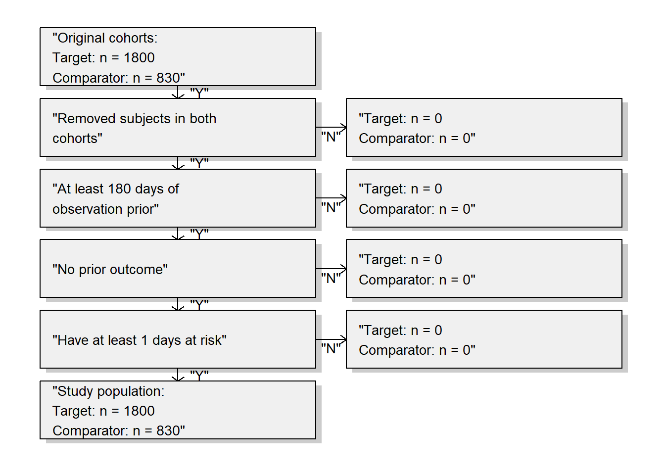
Create a study population using the createStudyPopulation function, requiring a 180-day washout period (minimum number of days of observation prior to first use), excluding people who had a prior outcome, and removing people that appear in both cohorts. Did we lose people?

studyPop <- CohortMethod::createStudyPopulation(
  cohortMethodData = cmData,
  outcomeId = 3,
  washoutPeriod = 180,
  removeDuplicateSubjects = "remove all",
  removeSubjectsWithPriorOutcome = TRUE,
  riskWindowStart = 0,
  startAnchor = "cohort start",
  riskWindowEnd = 99999)

Removing all subject that are in both cohorts (if any)

Requiring 180 days of observation prior index date

Removing subjects with prior outcomes (if any)

Removing subjects with less than 1 day(s) at risk (if any)

Study population has 2630 rows

CohortMethod::drawAttritionDiagram(studyPop)

No, we did not lose people. Probably because the restrictions used here were already applied in the cohort definitions.

Cox Proportional Hazards Model

The Cox Proportional Hazards Model is used to estimate a hazard ratio, which compares the risk of the outcome between different groups. In this study, we are comparing the risk of GI bleeding between users of celecoxib compared to users of diclofenac.

Book of OHDSI, Exercise 12.3

Fit a Cox proportional hazards model without using any adjustments. What could go wrong if you do this?

model <- CohortMethod::fitOutcomeModel(
  population = studyPop,
  modelType = "cox"
)

Using prior: None 
Using 1 thread(s)
Using 1 thread(s)
Using 1 thread(s)
Using 1 thread(s)
Using 1 thread(s)
Using 1 thread(s)
Using 1 thread(s)
Using 1 thread(s)

Fitting outcome model took 0.567 secs

Outcome model fitting status is: OK

model

Model type: cox
Stratified: FALSE
Use covariates: FALSE
Use inverse probability of treatment weighting: FALSE
Target estimand: ate
Status: OK

          Estimate lower .95 upper .95   logRr seLogRr
treatment  1.34612   1.10065   1.65741 0.29723  0.1044

A value of 1 would indicate no difference in risk, but our result is 1.346. This means the treatment group (celecoxib users) has a 34.6% higher risk of experiencing the event (GI bleeding) compared to the comparator group (diclofenac users).

The interval [1.10065, 1.65741] indicates that, with 95% confidence, the true hazard ratio lies within this range. Since the interval does not include 1, it suggests that the effect of the treatment is statistically significant at the 5% level.

It is likely that celecoxib users are not exchangeable with diclofenac users, and that these baseline differences already lead to different risks of the outcome. If we do not adjust for these difference, like in this analysis, we are likely producing biased estimates.

Fit a Propensity Model

Propensity Scores

Ideally, we would do a randomized trial to ensure no differences between the target and comparator cohorts that could confound your outcome. In a randomized trial, the probably of recieving each treatment would be 50%, given the set of all variables, including those which are not measured.

Unfortunately, this is often not possible, as we only have observational data and a set of measured variables, which is not exhaustive. However, we can use propensity scores to help adjust for confounders (things that influence the outcome apart from the exposures). This score is the probably of receiving the drug of interest conditioned on a number of measured characteristics on and before treatment initiation.

There are a few methods of using propensity scores to adjust for confounders. I will just cover matching and stratification.

Note

Propensity score adjustments are most effective when there are no unmeasured confounders. However, since this ideal condition is rarely met, it is misleading to claim that propensity score matching or stratification ‘mimics’ randomized trials.

PS Matching

Scenario: You are comparing the effect of Drug A and Drug B on recovery times for a condition.

1. Identify Covariates: Covariates include age, gender, and baseline health status.
2. Calculate Propensity Scores: Estimate the propensity scores for each patient based on these covariates.
3. Match Patients: Pair each patient receiving Drug A with a patient receiving Drug B who has the same propensity score.
   • Example:
     • Bilbo and Frodo both have a propensity score of 0.4 based on their measured characteristics.
     • Bilbo receives Drug A, and Frodo receives Drug B.
     • Both patients are included in the study because they have the same propensity score.
4. Compare Outcomes: For each patient receiving Drug A, find a matched patient receiving Drug B with the same propensity score and compare their recovery times.

PS Stratification

1. Identify Covariates: Covariates include age, gender, and baseline health status.
2. Calculate Propensity Scores: Estimate the propensity scores for each patient.
3. Create Strata: Divide patients into strata based on their propensity scores (e.g., low, medium, high).
   • Example:
     • Stratum 1: Propensity scores between 0.3 and 0.4.
     • Stratum 2: Propensity scores between 0.4 and 0.5.
     • Stratum 3: Propensity scores between 0.5 and 0.6.
4. Compare Within Strata: Compare the outcomes (recovery times) between Drug A and Drug B within each stratum.
   • Example:
     • In Stratum 1, where propensity scores range from 0.3 to 0.4, compare the average recovery times of patients on Drug A and Drug B.
     • Repeat the comparison for Stratum 2 and Stratum 3.

Overlap: Preference Scores

The preference score shows the distribution of propensity scores between two groups.

Basically, in order to do propensity score matching, there must be some overlap in the propensity scores for each group.

See this video about using preference scores for accessing the feasibility of comparative effectiveness research. This is also covered here in the Book of OHDSI.

Plot Preference Score Distribution

With that background established, let’s fit a propensity model and plot the preference scores. If there is sufficient overlap between the target and comparator cohorts, we can effectively compare them by adjusting for confounders through propensity score matching.

Book of OHDSI, Exercise 12.4

Fit a propensity model. Are the two groups comparable?

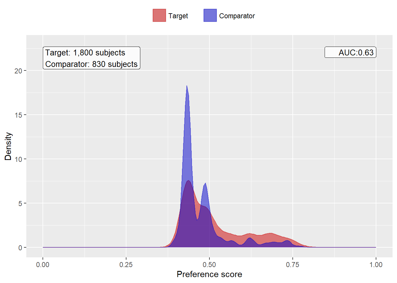
We fit a propensity model on our study population, using all covariates we extracted. We then show the preference score distribution:

ps <- CohortMethod::createPs(
  cohortMethodData = cmData,
  population = studyPop)

Removing 6 redundant covariates
Removing 112 infrequent covariates
Normalizing covariates
Tidying covariates took 1.94 secs
Propensity model fitting finished with status OK

Creating propensity scores took 10.1 secs

CohortMethod::plotPs(ps, showCountsLabel = TRUE, showAucLabel = TRUE)

Note that this distribution looks a bit odd, with several spikes. This is because we are using a very small simulated dataset. Real preference score distributions tend to be much smoother.

The propensity model achieves an AUC of 0.63, suggested there are differences between target and comparator cohort. We see quite a lot overlap between the two groups suggesting PS adjustment can make them more comparable. An AUC of 1 would mean that treatment assignment was perfectly predictable, so the two groups would not be comparable.

PS Stratification

Book of OHDSI, Exercise 12.5

Perform PS stratification using 5 strata. Is covariate balance achieved?

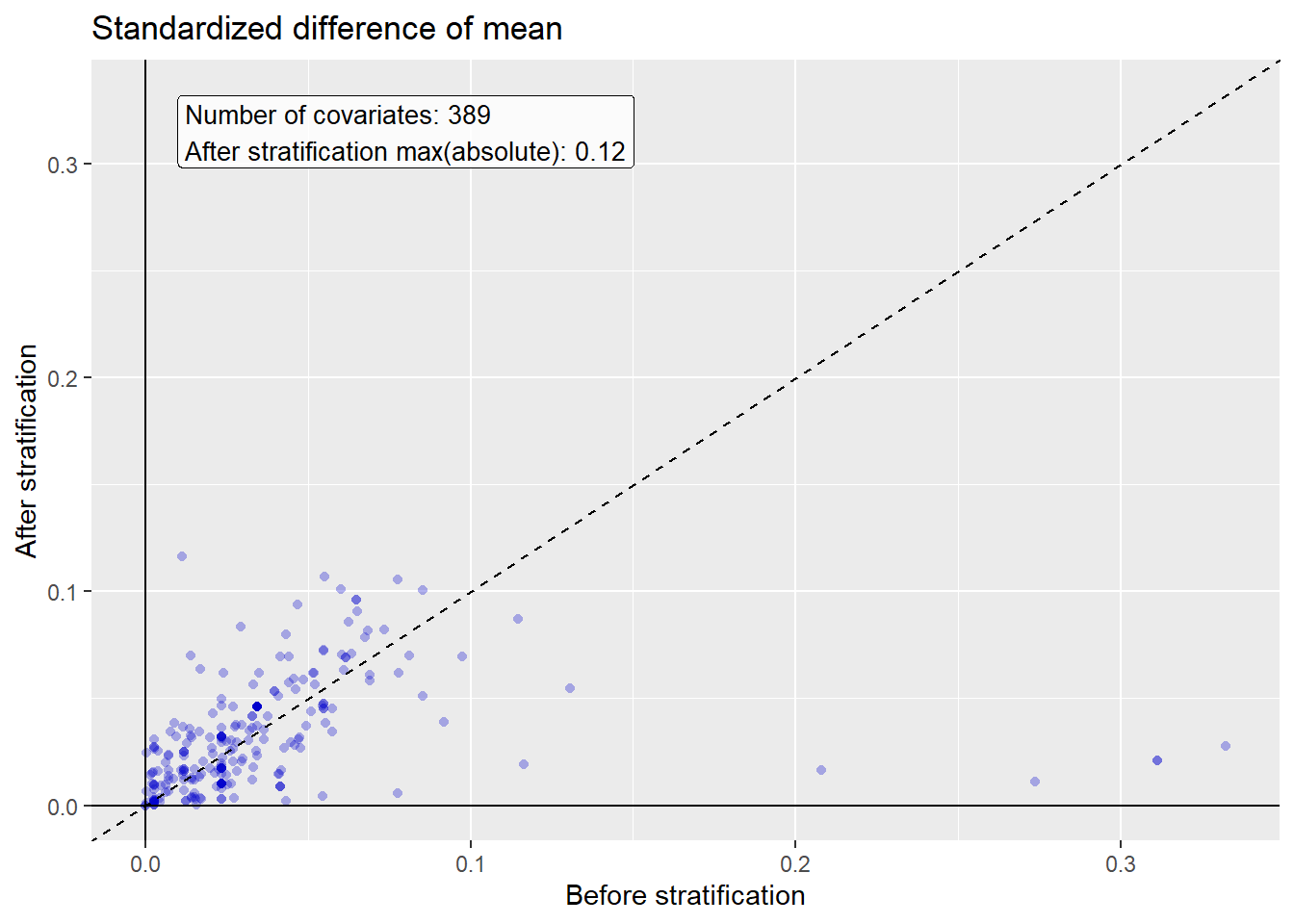
We stratify the population based on the propensity scores, and compute the covariate balance before and after stratification:

strataPop <- CohortMethod::stratifyByPs(ps, numberOfStrata = 5)
bal <- CohortMethod::computeCovariateBalance(strataPop, cmData)

Computing covariate balance took 2.42 secs

CohortMethod::plotCovariateBalanceScatterPlot(
  bal,
  showCovariateCountLabel = TRUE,
  showMaxLabel = TRUE,
  beforeLabel = "Before stratification",
  afterLabel = "After stratification"
)

Warning: Removed 139 rows containing missing values or values outside the scale range
(`geom_point()`).

We see that various baseline covariates showed a large (>0.3) standardized difference of means before stratification (x-axis). After stratification, balance is increased, with the maximum standardized difference <= 0.1.

Fit Cox Proportional Hazards Model using PS strata

Book of OHDSI, Exercise 12.6

Fit a Cox proportional hazards model using the PS strata. Why is the result different from the unadjusted model?

We fit a outcome model using a Cox regression, but stratify it by the PS strata:

adjModel <- CohortMethod::fitOutcomeModel(
  population = strataPop,
  modelType = "cox",
  stratified = TRUE
)

Using prior: None 
Using 1 thread(s)
Using 1 thread(s)
Using 1 thread(s)
Using 1 thread(s)
Using 1 thread(s)
Using 1 thread(s)
Using 1 thread(s)
Using 1 thread(s)

Fitting outcome model took 0.687 secs

Outcome model fitting status is: OK

adjModel

Model type: cox
Stratified: TRUE
Use covariates: FALSE
Use inverse probability of treatment weighting: FALSE
Target estimand: ate
Status: OK

          Estimate lower .95 upper .95   logRr seLogRr
treatment  1.10267   0.89758   1.36341 0.09773  0.1066

We see the adjusted estimate of 1.102 is lower than the unadjusted estimate of 1.346, and that the 95% confidence interval now includes 1. This is because we are now adjusting for baseline differences between the two exposure groups, thus reducing bias.

Thus, after adjusting for confounders using PS stratification, we conclude that there is not a significant difference in the risk of GI between users of celecoxib and users of diclofenac.